
Equipment maintenance DX by sensor data × data analysis
Part 3: Data Analysis for Achieving Predictive Maintenance - Method Using the Normal Distribution (1)
In the second article of the "Equipment Maintenance DX by Sensor Data × Data Analysis" series, we explained the data analysis techniques used in predictive maintenance and how to proceed with data analysis. By combining this with the content of the first article, the reader should be able to grasp the important points of combining predictive maintenance and data analysis. The "Equipment Maintenance DX by Sensor Data × Data Analysis" series covers content specializing in data science that explains common data analysis methods used in predictive maintenance. This third article of the series highlights Hotelling's T-squared method, a simple and powerful method that uses the normal distribution.
Introduction - Structure of This Article
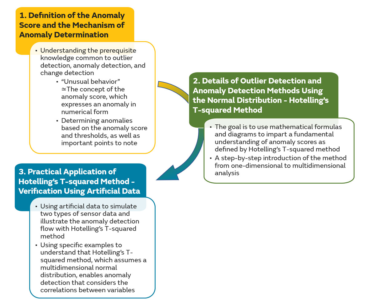
The structural flow of this article is shown in Figure 1. Section 1 focuses on content common to the methods introduced in this series. While mathematical formulas are used at times to dive into the details of the methods, we provide an easy-to-understand explanation of the mechanism and practical application of Hotelling's T-squared method through specific examples using conceptual diagrams and artificial data.
1. Definition of the Anomaly Score and the Mechanism of Anomaly Determination
The methods for outlier detection, anomaly detection, and change detection covered in this article and subsequent articles all share the common objective of selectively identifying data points or sets of data points that demonstrate "unusual behavior" as outliers, anomalies, and changes (see Part 2 for the concepts of outlier detection, anomaly detection, and change detection). To implement this as a method, we must effectively quantify and convert the concept of "unusual behavior," or anomalies, into numbers.
The indicator that quantifies and converts anomalies into numbers is generally referred to as an "anomaly score." An anomaly score is defined as a numerical indicator that takes a positive value and indicates the degree to which a certain data point or set deviates from the data points or set said to represent normal behavior (normal data) (Figure 2). The introduction of anomaly scores makes it possible to intuitively understand that if the anomaly score of a certain set of data is low, it indicates behavior similar to the norm, while a high score indicates an anomaly. While the definition of an anomaly score differs depending on the method used, the meaning is consistent with the explanation above.
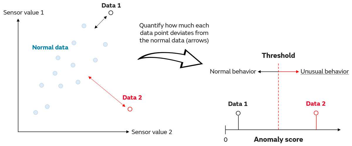
In order to conclusively determine if the data is normal or anomalous using the anomaly score, it is necessary to set an anomaly score threshold that separates the two results (Figure 2, right). While there are various methods for setting the threshold, they are often also decided based on the user's specific requirements (Column 1: Evaluation Metrics for Outlier Detection, Anomaly Detection, and Change Detection Methods). An important point to recognize is that there are fundamentally no universally applicable threshold criteria that can be used across all methods as values must be set by the user according to the situation.
The points described above are the absolute minimum for understanding the individual methods for outlier detection, anomaly detection, and change detection. With these points in mind, the next section will examine the details of a representative method that uses the normal distribution for outlier detection and anomaly detection.
2. Details of Outlier Detection and Anomaly Detection Methods Using the Normal Distribution - Hotelling's T-squared Method
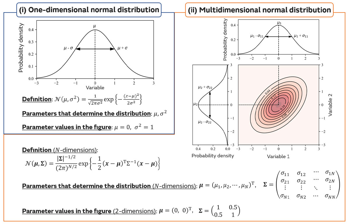
The method of outlier detection and anomaly detection using the normal distribution is called "Hotelling's T-squared method." This method defines the anomaly scores and sets the thresholds by assuming that the normal data at hand follows a one-dimensional normal distribution (Figure 3-(i)) for one-dimensional data and a multidimensional normal distribution (Figure 3-(ii)) for multidimensional data.
In this section, we first explain Hotelling's T-squared method using a one-dimensional normal distribution*1, which we then use to extend the explanation to a multidimensional normal distribution*1. Finally, we present the advantages and disadvantages of this method in practical use. This section is structured so you can gain a deeper understanding of the method by reading it step by step.
*1 The one-dimensional normal distribution and multidimensional normal distribution are also referred to as the "univariate normal distribution" and "multivariate normal distribution."
2.1 Anomaly Scores and Thresholds in a One-Dimensional Normal Distribution
Let us assume that the one-dimensional normal data follows a one-dimensional normal distribution (Figure 3-(i)). Based on the properties of the normal distribution, the normal data in this case consists of values centered around 𝜇 with a spread of approximately 𝜎. The normal distribution parameters 𝜇 and 𝜎 must be estimated in advance from the normal data at hand.
Based on the assumptions above, the anomaly score 𝑎(𝑥) at a certain data point 𝑥 can be defined according to Equation (1). Figure 4 also shows a specific example which explains the anomaly score concept.

In Figure 4, the two types of normal data are assumed to follow normal distributions 𝒩₁, 𝒩₂. Below, we aim to explain the anomaly score metric and the threshold concept using examples where data points 𝑥₁ and 𝑥₂ exist with respect to each distribution. In this example, 𝑥₂ is assumed to be normal data, while 𝑥₁ is anomalous.
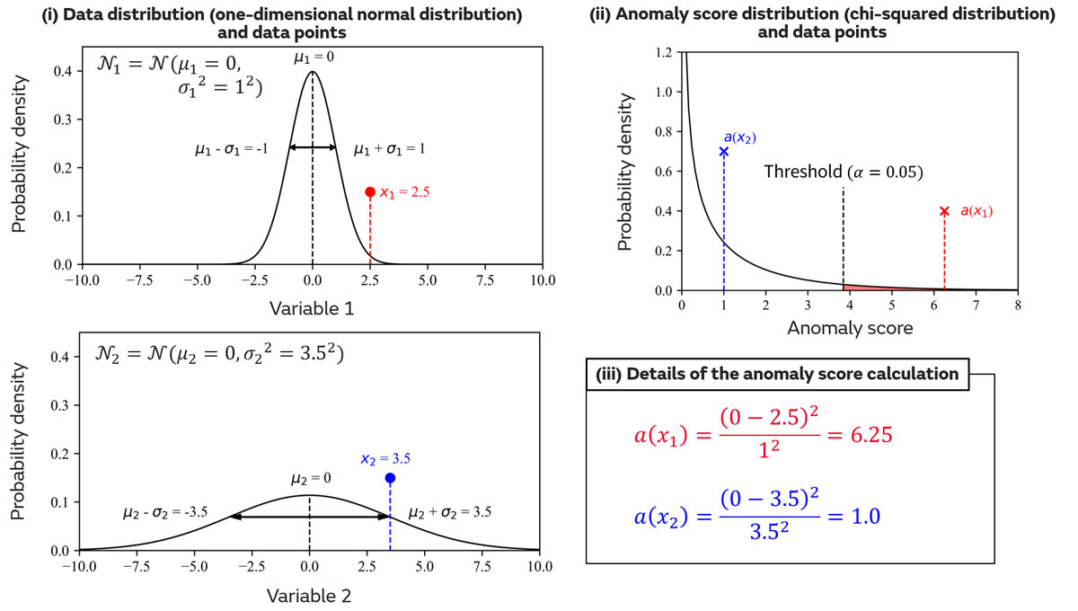
From Figure 4-(i) and Equation (1), we can understand that the numerator of the anomaly score corresponds to the distance between a given data 𝑥 and the center 𝜇 of the normal distribution to which the normal data conforms. This term quantifies "something that differs from the norm" in a straightforward manner. However, the numerator alone does not take into account the spreads 𝜎₁ and 𝜎₂ of the normal distribution*2. The denominator plays the role of effectively accounting for this characteristic. The results of actually calculating the anomaly scores for 𝑥₁ and 𝑥₂ are shown on the right side of Figure 4. As expected, the anomaly score for 𝑥₁ is extremely large when compared to the score for 𝑥₂. This clearly shows that the anomaly score effectively takes the distribution spread into account.
To set the threshold, we can take advantage of the fact that the anomaly score itself follows a probability distribution consisting of either an F-distribution with (1, 𝑛−1) degrees of freedom or a chi-squared distribution (Column 2: Chi-squared Distribution and F-distribution) with one degree of freedom. The 𝑛 variable appearing in the degrees of freedom of the F-distribution corresponds to the number of normal data points used to estimate the parameters 𝜇 and 𝜎.
Figure 3-(ii) shows a chi-squared distribution with one degree of freedom, which the anomaly score follows approximately, and its shape shows that the probability density decreases as the anomaly score increases. In other words, data with a high anomaly score can be interpreted as a rare event that only occurs with an extremely low probability. When using a probability distribution, the threshold for identifying it as an anomaly is set based on the degree of rarity of the data's anomaly score, or in other words, its probability of occurrence.
As previously mentioned, there is no universally applicable threshold, and the appropriate value must be set according to the problem. Conventionally, the upper 5% or 1% levels*3 of the chi-squared distribution are often used and notated as 𝛼=0.05 or 𝛼=0.01. The example shown in Figure 4-(ii) adopts the upper 5% level as the threshold. If the anomaly value of a certain data set exceeds this level (red area in Figure 4-(ii)), that data is determined to be an anomaly.
While the explanation above describes how to use probability distributions to set thresholds, there are various other methods such as quantiles (e.g., the upper 1% point) that use the magnitude of the anomaly scores themselves.
*2 If only the numerator is defined as the anomaly score, we get the contrary result that data point 𝑥₂ is more anomalous.
*3 These correspond to the values on the chi-squared distribution where the probability of data exhibiting that specific anomaly score occurring is 5% or 1%.
2.2 Anomaly Scores and Thresholds in a Multidimensional Normal Distribution
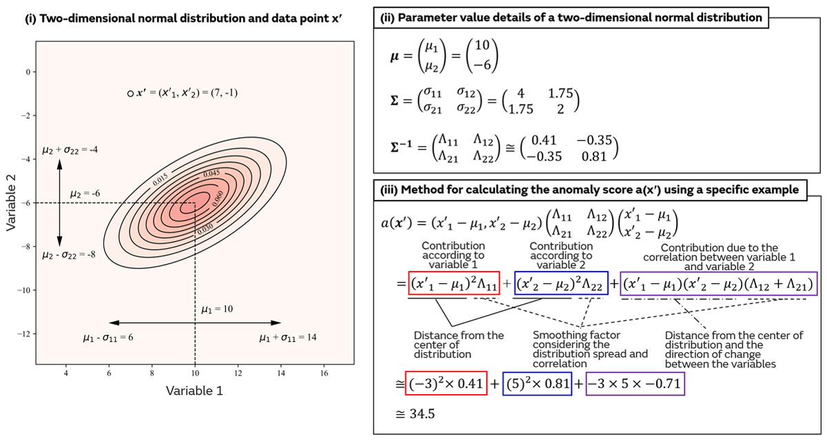
When the normal data is multidimensional (𝑁>1), the equation becomes more complex, but the approach itself does not change very much from the one-dimensional case. Assuming that the data dimension is 𝑁-dimensions and the normal data follows a multidimensional normal distribution, estimate the parameters 𝝁 and 𝚺⁻¹ in advance from the available normal data. At this time, the anomaly score of a set of data points 𝒙=(𝑥₁, 𝑥₂, ⋯, 𝑥𝑁)T is defined as follows.

Similar to Equation (1), Figure 5 shows a specific example of the calculation of Equation (2) (𝑁=2). The (𝒙−𝝁) that appears twice in Equation (2) corresponds to the numerator of Equation (1), 𝚺⁻¹ corresponds to the denominator term of Equation (1), and their meanings are almost the same as in Equation (1). We wrote that the denominator term in Equation (1) plays the role of smoothing the spread of the distribution. In addition, the denominator of Equation (2) smooths the information so that it can be integrated even if the units of the elements that make up data point 𝒙 are different*4, and it also functions to effectively reflect the effect of any correlations between each element. This can be clearly understood by performing a specific calculation. If you are interested in the details of the calculation, refer to the calculation examples in Figure 5-(ii) and (iii). In particular, the discussion of the correlation effect will be explained once again with specific examples using artificial data in Section 3 of Part 3 (2).
The steps after calculating the anomaly score are exactly the same as in the one-dimensional example. The only difference is the degrees of freedom of the probability distribution. For a multidimensional normal distribution, the anomaly score follows either an F-distribution with degrees of freedom (𝑁, 𝑛−𝑁) or a chi-squared distribution with degrees of freedom 𝑁 (Column 2: Chi-squared Distribution and F-distribution). The 𝑛 that appears in the degrees of freedom of the F-distribution corresponds to the number of normal data points used in the estimation of 𝝁 and 𝚺⁻¹.
*4 For example, when 𝒙=(𝑥₁, 𝑥₂)T, we assume that 𝑥₁ is the vibration sensor value and 𝑥₂ is the temperature sensor value. Although the units and possible range of numerical values are completely different, the denominator of Equation (2) lets us calculate an anomaly score that takes these two values into account. An example of such a calculation is shown in Figure 5 and in Section 3 of Part 3 (2).
2.3 Advantages and Disadvantages of Hotelling's T-squared Method
So far, we have explained the details of Hotelling's T-squared method, and the advantages and disadvantages relating to practical application are summarized in Table 1 below. Countermeasures are also listed for the disadvantages.
| Advantages | ・The mechanism behind the method is clear, and the results are easy to interpret. ・Able to handle multidimensional data and take into accounts its correlation structure. |
|---|---|
| Disadvantages | ・Performance degrades if the normal data does not follow a normal distribution (e.g., a multimodal distribution) or if extreme outliers are present. ・Performance degrades if the number of dimensions is too high relative to the number of data points (curse of dimensionality). ・Unable to calculate which variable had a significant impact when an anomaly occurs. |
| Countermeasures for the disadvantages | ・Consider the application of more flexible methods (e.g., multimodal distribution: Gaussian Mixture Model (GMM)) or remove the outliers from the normal data through preprocessing. ・Delete unnecessary variables in advance or avoid the curse of dimensionality through dimension reduction (e.g., Principal Component Analysis (PCA) and Partial Least Squares (PLS) Regression) ・Use methods that can calculate the contribution of each variable to the anomaly (e.g., Mahalanobis-Taguchi method) |
Column 1: Evaluation Metrics for Outlier Detection, Anomaly Detection, and Change Detection Methods
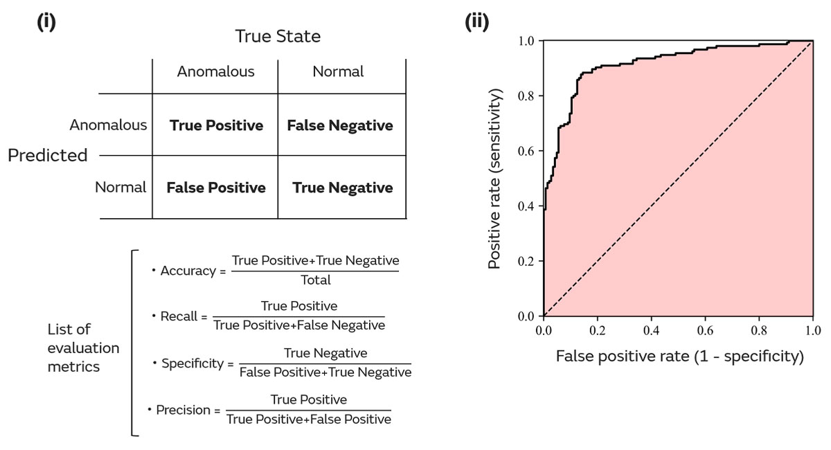
While qualitative judgments can be made by visually inspecting results of outlier detection, anomaly detection, and change detection, quantitative evaluation of the results is equally important. Evaluation metrics are essential for quantitatively evaluating the results. Figure 6 shows a representative evaluation metric used in outlier detection, anomaly detection, and change detection.
Using such evaluation metrics offers significant benefits, such as allowing for the definition of target goals, facilitating smooth communication with predictive maintenance stakeholders, and enabling the comparison of results obtained with different methods, etc.
At the same time, caution is required regarding the need to use evaluation metrics that can appropriately evaluate the points that you wish to quantitatively assess in predictive maintenance. Figure 6 shows commonly used metrics, but the question of which evaluation metric to use should be decided on a case-by-case basis. When selecting an evaluation metric, it is important to reaffirm the objectives of predictive maintenance and what must be evaluated to achieve those objectives as well as check what metrics are being used in similar cases. You should also recognize the option of creating your own evaluation metrics and using them for evaluation if necessary.
Column 2: Chi-squared Distribution and F-distribution
The chi-squared distribution and F-distribution, which appear as the distributions followed by the anomaly scores in Hotelling's T-squared method, possess the following properties.
[Chi-squared Distribution] (chi is the letter 𝜒 from the Greek alphabet)
If a random variable 𝑧 follows a standard normal distribution*5, the sum of squares of 𝑚 variables 𝑧𝑖(𝑖=1~𝑚) independently obtained from that distribution is defined as following a chi-squared distribution with 𝑚 degrees of freedom as shown below.

*5 Refers to the normal distribution denoted by 𝒩(𝜇=0, 𝜎²=1). A variable 𝑥 that follows any normal distribution 𝒩(𝜇, 𝜎²) can be converted into a variable 𝑧 that follows the standard normal distribution through an operation called standardization as shown in Equation (3) below.

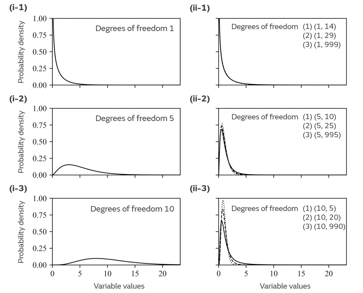
The number of degrees of freedom is a parameter that determines the shape of the distribution. The shape of the chi-squared distribution when the degrees of freedom are varied is shown in Figure 7-(i).
The chi-squared distribution is used in goodness-of-fit tests and tests of independence, etc. In Hotelling's T-squared method, the anomaly score can be assumed to approximately follow the chi-squared distribution if the number of normal data points 𝑛 is sufficiently large.
[F-distribution]
If random variables 𝑢 and 𝑣 follow chi-squared distributions with mutually independent 𝑝 and 𝑞 degrees of freedom (𝑢~𝜒𝑝², 𝑣~𝜒𝑞²), then the F-distribution with 𝑝 and 𝑞 degrees of freedom is defined as follows.

The number of degrees of freedom is a parameter that determines the shape of the distribution. The shape of the F-distribution when the degrees of freedom are varied is shown in Figure 7-(ii).
The F-distribution is used in applications such as the F-test to determine whether the variances of two data sets are equal. In Hotelling's T-squared method, it may be assumed that the numerical value obtained by multiplying the anomaly score by an appropriate scale factor follows an F-distribution.